Basic Tutorial#
This notebook shows the most basic features of Metadensity
[1]:
# set up files associated with each genome coordinates
import metadensity as md
md.settings.from_config_file('/home/hsher/projects/Metadensity/config/hg38.ini')


# then import the modules
from metadensity.metadensity import *
from metadensity.plotd import *
import pandas as pd
import matplotlib.pyplot as plt


# I have a precompiles list of ENCODE datas as a csv that loads in this dataloader
import sys
sys.path.append('/home/hsher/projects/Metadensity/scripts')
from dataloader import *
%matplotlib inline

plt.style.use('seaborn-white')
please set the right config according to genome coordinate
Using /home/hsher/gencode_coords/GRCh38.p13.genome.fa
Using:  /home/hsher/gencode_coords/gencode.v33.transcript.gff3
Load encode metadata#
I have precompiled list of uID and the .bam, .bigWig files in the following dataframe.
minus_0 is the bigWig file for minus strand for replicate 0. The files are in /home/hsher/seqdata/eclip_raw. You don’t need to specify all of them. The eCLIP object will take care of them.
load RBPs into eCLIP object#
I build an eCLIP object that will connect all .bam, .bigWig and .bed (for IDR peaks, individual peaks) together. All you need to do is point a row of the previous dataframe, and use RBP_centric_approach() to compute the regions for metagene, and find positive (transcripts with IDR) and negative (transcript w/o any peaks) examples. Building the object will take a while (~1 min) since a lot of I/O.
[2]:
HNRNPC = eCLIP.from_series(encode_data.loc[(encode_data['RBP'] == 'HNRNPC')&(encode_data['Cell line'] == 'HepG2')].iloc[0],
                          single_end = False)
[3]:
RPS3 = eCLIP.from_series(encode_data.loc[(encode_data['RBP'] == 'RPS3')&(encode_data['Cell line'] == 'HepG2')].iloc[0],
                        single_end = False)
[4]:
RBFOX2 = eCLIP.from_series(encode_data.loc[(encode_data['RBP'] == 'RBFOX2')&(encode_data['Cell line'] == 'HepG2')].iloc[0],
                          single_end = False)
[5]:
LIN28B = eCLIP.from_series(encode_data.loc[(encode_data['RBP'] == 'LIN28B')&(encode_data['Cell line'] == 'HepG2')].iloc[0],
                          single_end = False)
Calulcate Density and Truncation sites#
Object Metatruncation and Metadensity takes three things: 1. an experiment object eCLIP or STAMP. 2. a set of transcript pyBedTools that you want to plot on 3. name of the object
Options include: 1. sample_no= allows you to decide how many transcript you want to build the density. It will take longer. By default, sample_no=200. So in transcript if you give more than 200 transcripts, only 200 will be used 2. metagene allows you to use pre-built metagene. This feature is more useful when you want to compare the same set of RNA over many RBPs. 3. background_method handles how you want to deal with IP v.s. Input 4. normalize handles how you want to
normalize values within a transcript.
Difference between truncation and density#
Metadensity represents read coverage. Metatruncation represents the 5’ end of read 2 for eCLIP; edit sites for STAMP.
[6]:
# here for the set of transcript, we use the IDR peak containing transcript assuming they have good signal
def build_idr_metadensity(eCLIP):
    ''' build metadensity object for eCLIP and its idr peak containing transcript'''
    m = Metadensity(eCLIP, eCLIP.name,background_method = 'subtract', normalize = True)
    m.get_density_array()
    return m
def build_idr_metatruncate(eCLIP):
    ''' build metadensity object for eCLIP and its idr peak containing transcript'''
    m = Metatruncate(eCLIP, eCLIP.name,background_method = 'subtract', normalize = True)
    m.get_density_array(use_truncation = True)
    return m
[7]:
# this step takes some time for building metagene from the annotation files.
HNRNPC_den = build_idr_metadensity(HNRNPC)
RPS3_den = build_idr_metadensity(RPS3)
RBFOX2_den = build_idr_metadensity(RBFOX2)
LIN28B_den = build_idr_metadensity(LIN28B)

HNRNPC_trun = build_idr_metatruncate(HNRNPC)
RPS3_trun = build_idr_metatruncate(RPS3)
RBFOX2_trun = build_idr_metatruncate(RBFOX2)
LIN28B_trun = build_idr_metatruncate(LIN28B)
Using: /home/hsher/projects/Metadensity/metadensity/data/hg38/gencode
Done building metagene
Using: /home/hsher/projects/Metadensity/metadensity/data/hg38/gencode
Done building metagene
Using: /home/hsher/projects/Metadensity/metadensity/data/hg38/gencode
Done building metagene
Using: /home/hsher/projects/Metadensity/metadensity/data/hg38/gencode
Done building metagene
need at least one array to concatenate
Using: /home/hsher/projects/Metadensity/metadensity/data/hg38/gencode
Done building metagene
Using: /home/hsher/projects/Metadensity/metadensity/data/hg38/gencode
Done building metagene
Using: /home/hsher/projects/Metadensity/metadensity/data/hg38/gencode
Done building metagene
Using: /home/hsher/projects/Metadensity/metadensity/data/hg38/gencode
Done building metagene
need at least one array to concatenate
Visualize RBP map: individual density per transcript#
[8]:
from metadensity.plotd import *
[9]:
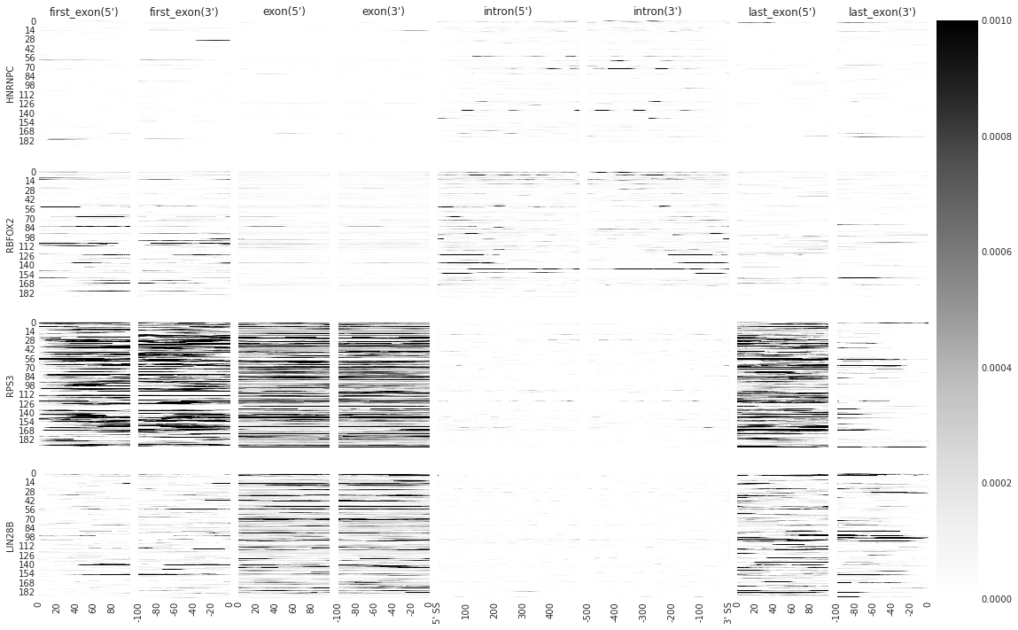
### PLOT INDIVIDUAL DENSITY
# you can customize the list of features you want to show. This is suitable when you are looking for splicing
f = plot_rbp_map([HNRNPC_den,  RBFOX2_den, RPS3_den,LIN28B_den], features_to_show = generic_rna)
/projects/ps-yeolab3/hsher/Metadensity/metadensity/plotd.py:187: RuntimeWarning: Mean of empty slice
  density_concat = np.nanmean(np.stack([den_arr[feat,align, r] for r in m.eCLIP.rep_keys]), axis = 0)
[10]:
### PLOT INDIVIDUAL TRUNCATION SITES

#f = plot_rbp_map([HNRNPC_trun,  RBFOX2_trun, RPS3_trun,LIN28B_trun], features_to_show = generic_RNA)
Median and Mean density over many transcripts#
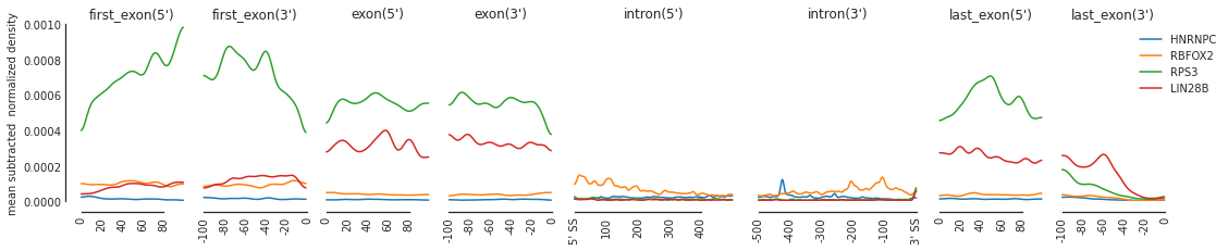
[11]:
color_dict = {'HNRNPC':'dodgerblue', 'RBFOX2':'darkorange', 'RPS3':'green', 'LIN28B':'red'}
%matplotlib inline
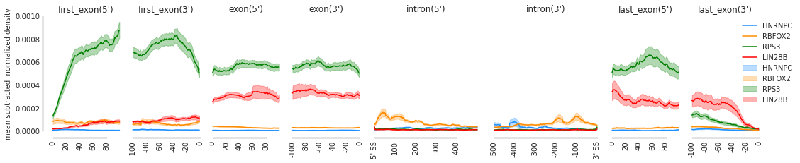
f=plot_mean_density([HNRNPC_den, RBFOX2_den, RPS3_den, LIN28B_den],
features_to_show = generic_rna, ymax = 0.001,
color_dict = color_dict)
f = beautify(f)
[12]:
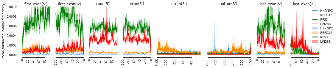
f=plot_mean_density([HNRNPC_trun, RBFOX2_trun, RPS3_trun, LIN28B_trun],
                    features_to_show = generic_rna, ymax = 0.001,
                   color_dict = color_dict)
f = beautify(f)
[13]:
# you can smooth if you find spiky truncation density ugly :-\
f=plot_mean_density([HNRNPC_trun, RBFOX2_trun, RPS3_trun, LIN28B_trun], features_to_show = generic_rna, ymax = 0.001, smooth = True)
f = beautify(f)
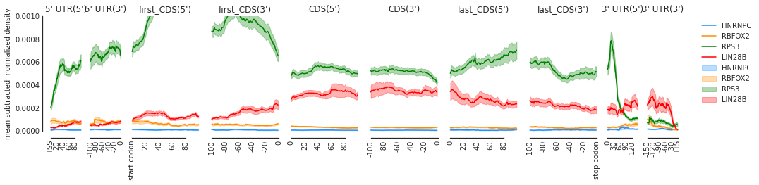
[14]:
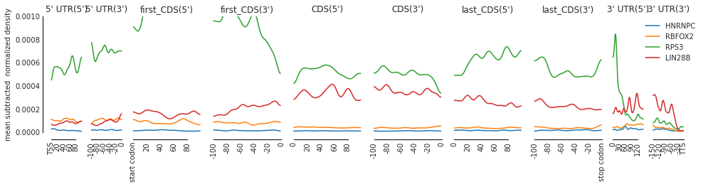
f=plot_mean_density([HNRNPC_den, RBFOX2_den, RPS3_den, LIN28B_den], features_to_show = protein_coding, ymax = 0.001, color_dict = color_dict)
f = beautify(f)
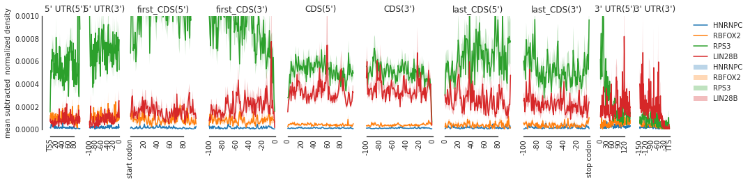
[15]:
f=plot_mean_density([HNRNPC_trun, RBFOX2_trun, RPS3_trun, LIN28B_trun], features_to_show = protein_coding, ymax = 0.001)
f = beautify(f)
[16]:
f=plot_mean_density([HNRNPC_trun, RBFOX2_trun, RPS3_trun, LIN28B_trun],
                    features_to_show = protein_coding, smooth = True, ymax = 0.001)
f = beautify(f)